
by Darrell
7 October 2014
The Problem With Fuel Cell Models
Darrell Teegarden
www.linkedin.com/in/darrellteegarden
Performing a web search for "fuel cell model" returns an encouraging number of hits. When these are pursued, however, it is difficult to find the result that many engineers are looking for -- a model of a fuel cell that can quickly and easily be used to explore the behavior of an existing, commercial fuel cell in the context of an electronic circuit.
What is found instead are technical papers that are largely focused on how a fuel cell works, often at a physics level that requires knowledge of the fuel cell's construction. Other search results may provide model information that is at the right behavioral level but that is in a form that is difficult to use. This is either because they are presented only in their theoretical form -- without a convenient way to execute them -- or because the target execution environment is proprietary (e.g., university) and/or commercially expensive.
SPICE is a common circuit simulation environment, good for modeling much of the rest of the circuits of interest that surround a fuel cell, but it comes up short without availability of a good fuel cell model.
What follows is the presentation of a model that solves all of these problems. The model presented is theoretical, but with a free, open, online execution model written in VHDL-AMS. The model can be used to fit available polarization curves, so that a commercial fuel cell can be modeled without knowing the details of how it is constructed. Finally, the model can be used in arbitrary PartQuest Explore circuit schematics, available free and online on PartQuest Explore.
Because it is built upon VHDL-AMS, PartQuest Explore has all the advantages of a SPICE circuit simulator, a VHDL digital simulator, a block-diagram / control systems simulator, and a multi-physics system simulator, all in one convenient, graphical environment.
Modeling a Fuel Cell in the PartQuest Explore Design Environment
This blog entry provides an overview of hydrogen PEM fuel cells, presents the theoretical equations needed to model a fuel cell for use in circuit applications, and demonstrates the implementation of a basic fuel cell model using the VHDL-AMS modeling language.
Links are provided, below, to pages on the explore.partquest.com site that allow you to experiment with this model yourself, in circuits that exercise the fuel cell in the context of various systems.
Fuel Cell Structure
Hydrogen fuel cells, as shown in Figure 1, are electrochemical devices that run on hydrogen and produce electrical power. They are environmentally friendly because heat and water are the only byproducts. They can be used in a variety of applications including transportation, stationary power generation, and portable devices. See this Wikipedia article for more information.
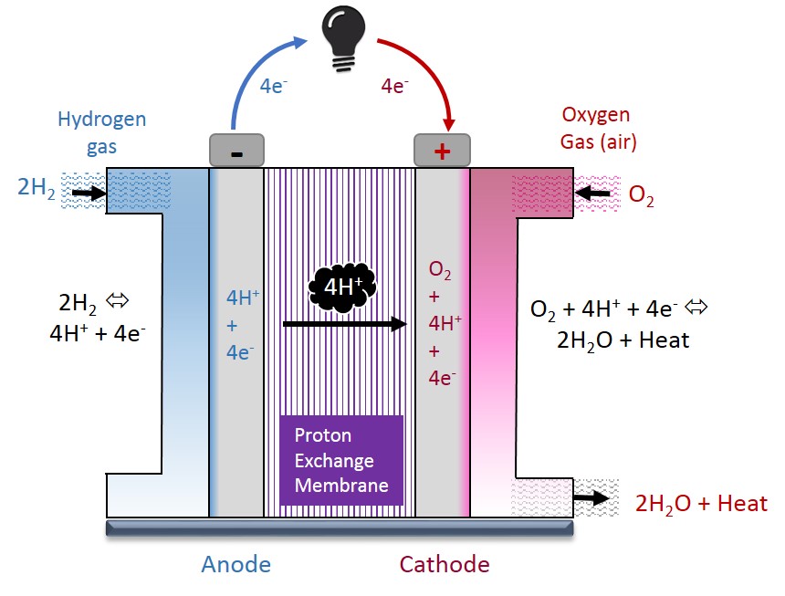
Figure 1. Fuel Cell Diagram[1]
Modeling is a useful technique that allows important variables to be parameterized and provides visibility to the key factors that drive performance. By pinpointing areas of improvement through modeling, the process of optimizing fuel cells—and the systems in which they operate— becomes more focused, accurate, and cost effective.
Modeling a Fuel Cell
The electrochemical behavior of a fuel cell is primarily defined by the so-called polarization curve, which is a plot of fuel cell output voltage as a function of load current. Under no-load conditions, a fuel cell operates at the ideal thermodynamic voltage (sometimes referred to as electromotive force or EMF). In practical loading conditions, however, the losses characterized by the polarization curve are of first-order importance.
There are three primary operating regions on the polarization curve; these regions relate to different processes that are central to the fuel cell’s performance (and energy losses):
- The first loss that appears is the activation loss, which dominates at lower current densities and is related to the finite rate of reaction of both hydrogen and oxygen.
- The next area of loss is the ohmic loss, which is caused by electron and proton transport.
- The third loss, mass transport loss, dominates at higher current densities and is related to a finite supply of hydrogen and oxygen reactants and/or an uneven concentration of these reactants.
Reducing these losses and optimizing the components for the loads presented by the system will help improve the performance of the fuel cell.
Fuel Cell Equations
Fundamentally, the fuel cell model behaves as a voltage source where the voltage is dependent on the current supplied by the fuel cell source [3]. See Table 1., below, for a description of all of the variables, coefficients, and constants.
| Symbol | Description | Units |
Type |
Typical value |
|---|---|---|---|---|
| Fuel cell current | ampere | Independent | 0 - 600 A | |
| Fuel cell temperature | kelvin | Independent | 300 K | |
| Fuel cell terminal voltage, relative to reference terminal | volt | Dependent | 0 - 400 V | |
| Fuel cell open circuit (zero load current) voltage for a single cell | volt | Coefficient | 1.2 V | |
| Activation voltage drop, without considering time-dependent charge dynamics | volt | Dependent | < |
|
| Activation voltage drop, including time-dependent charge dynamics | volt | Dependent | < |
|
| Voltage drop due to fuel cell internal resistance | volt | Dependent | < |
|
| Voltage drop due to reactant mass transport across the fuel cell | volt | Dependent | < |
|
| Activation voltage reaction rate variable | volt | Dependent | ||
| Exchange current density | ampere | Coefficient | 50 A | |
| Universal gas constant | Constant | 8.3144621 |
||
| Number of electrons involved in electrochemical reaction | unit less | Constant | 2 | |
| Charge transfer coefficient | unit less | Coefficient | 0.2 | |
| Faraday's constant | Constant | 96485.3399 |
||
| Fuel cell internal resistance | Coefficient | 0.9 m |
||
| Empirical coefficient for transport loss | volt | Coefficient | 30 mV | |
| Empirical coefficient for transport loss | Coefficient | 0.015 |
||
| Time delay for activation voltage drop | second | Coefficient | 1 s | |
| Laplace transform variable "s" | Operator | N/A | ||
| The number of series-connected cells that comprise the fuel cell stack | unit less | Constant | 300 |
Table 1. Variables, coefficients, and constants
The time-varying, current-dependent voltage of the fuel cell, , is determined by starting with the ideal open-circuit voltage,
, and subtracting the three dominant loss effects, which are modeled as current-dependent (
) voltage drops. The open circuit voltage of the cell depends primarily on the chemistry of the cell (hydrogen-oxygen, for example).
Now we will examine each of these losses in more detail.
Activation Loss
Instantaneous behavior
The activation portion of the polarization curve is modeled using the Tafel equation. When time-dependent effects are ignored, and when the cell current () is greater than exchange current density (
), the instantaneous activation voltage drop is described below :
This instantaneous activation voltage drop is zero for cell currents less than . The coefficient
models the effective reaction rate in the fuel cell (how fast the reactions are occurring or how fast the reactants are entering the membrane), with higher values for an electrochemical reaction that is slow. The constant
is normally a function of temperature (
) and can be represented by the following function:
R and F are constants (ideal gas constant and Faraday’s constant, respectively), T is the temperature of the cell, z is the number of moving electrons, and is the constant exchange current coefficient. Empirical tests performed on fuel cells have demonstrated that
(the exchange current density; i.e., the current in either direction under reversible conditions) has a greater impact on fuel cell performance than the coefficient A [3].
Time-dependency
The activation voltage drop, in real fuel cells, does not react instantly to changes in load current. This is related to charge storage in the cells. This effect can be modeled easily by introducing a simple time delay, , between the desired activation voltage (
), and the activation voltage that would be observed if the cells were able to respond instantaneously (
). This can be included in the model by using either a Laplace domain equation for approximating the delay, or an equivalent differential equation form.
The transfer function in the Laplace domain looks like this:
The equivalent relationship in the time domain, as a differential equation, looks like this:
Ohmic Loss
The ohmic resistance loss is a simply a constant internal resistance formed by the conductance path through the cell.
Transport Loss
The mass transport loss is modeled from the empirical data available using two constants, m and n, that model the drop in the fuel cell voltage at higher currents.
Modeling Multiple Cells in a Stack
The above equations model a single cell of a fuel cell stack. There are typically hundreds of cells, connected in series, to provide enough power and high enough voltages for practical applications. Modeling of multiple cells can be accomplished by connected the appropriate number of cells in a series circuit. It is more convenient for users of the model, as well as more computationally efficient, to simply multiply each cell voltage by the number of cells in the stack ()
Model Validation
Before using this fuel cell model in a circuit or system application, it is important to first validate it. To accomplish this, the model is simulated in the PartQuest Explore simulator, right here on PartQuest Explore. For your convenience, and to improve clarity, a version of each design used to validate the model has been embedded directly in this blog. If you move your mouse over any of these designs, you will notice that it's live! Try interacting with the design to examine it closer.
Polarization Curve
Figure 2. Validation of model polarization curve
Single fuel cell voltages are typically too low (< 1.2 Volts) to be used in a system individually, so they are usually deployed in a stack of multiple cells in series. The examples here use 300 cells in a series stack. This would be typical, for example, for a fuel cell vehicle application.
The graph in Figure 2. shows the fuel cell voltage under different current load conditions and displays the different losses that occur throughout the fuel cell, including the activation, ohmic, and concentration polarization losses. These can be seen in the curve inflections, at the low-current (activation), mid-current (ohmic), and high-current (concentration) regions of the curve.
Dynamic Step-Load Response
Likewise, a voltage versus time waveform is plotted from the transient load test schematic (Figure 3.). This shows the time-varying voltage that is supplied by the fuel cell to the load (time-varying resistance) during abrupt low-current / high-current transitions. This is for a fuel cell module with 300 cells in series. You can examine this design more closely here.
Figure 3. Validation of model dynamic response
Using the Model to Calculate Useful Quantities
The VHDL-AMS model includes the fundamental variables and the algebraic and differential equations, described above, needed to completely determine the behavior of the model in an arbitrary circuit. This model can be combined in circuits using any of the hundreds of other models that are available in the PartQuest Explore simulation environment. This is one of the most powerful aspects of the VHDL-AMS language and its implementation in the PartQuest Explore simulator. The model can also include variables and equations that, while not needed to uniquely specify the device being modeled, provide useful analysis and insight into the operation of the device in the context of the system simulation. Examples of these include the calculation of chemical reactants consumed in the fuel cell reaction, electrical power losses, and power efficiency of the fuel cell. It is convenient, for example, to see how many moles or kilograms of hydrogen are consumed under particular electrical power load conditions.
See Also
You can learn more about this model and circuits that are used in this blog by going to the following design links. For each of these circuit designs, you can directly probe more deeply into the operation of the design. Or, if you prefer, you can make a copy of the design and experiment with it more thoroughly, including changing parameter values. You can even completely modify the schematic for you own use.
You may also find the following related white paper to be interesting:
Acknowledgements
This blog entry is based upon a white paper entitled: A VHDL-AMS Fuel Cell Model for Mechatronic System Analysis, co-written by Darrell Teegarden, Mike Donnelly, and Vijay Edupuganti.
References
[1] Farrington, L. (Writer). (2003). Fuel for thought on cars of the future [Print Photo]. Retrieved from http://www.scientific-computing.com/features/feature.php?feature_id=126
[2] Ashenden, P., Peterson, G., & Teegarden, D. (2003). The System Designer's Guide to VHDL-AMS. San Francisco, CA: Morgan Kaufmann Publishers. Available on Amazon.com.
[3] Larminie, J., & Dicks, A. (2003). Fuel cell systems explained. (2nd ed.). London, England: Wiley.
Appendix: Fuel Cell VHDL-AMS Implementation
The following VHDL-AMS code is a direct implementation of the fuel cell equations, above. The VHDL-AMS language [2] is perfectly suited for this kind of modeling task, as the resulting model can so easily be used in broader circuit and system simulations, directly on the explore.partquest.com website.
Figure 5. Fuel cell VHDL-AMS model
library IEEE;
use IEEE.electrical_systems.all;
use IEEE.energy_systems.all;
use IEEE.math_real.all;
use IEEE.thermal_systems.all;
use IEEE.fluidic_systems.all;

library MGC_AMS;
use MGC_AMS.conversion.all;

entity fuel_cell_basic is

  generic (
    NCells        : positive          := 300;      -- Number of cells, in series,
                                                   -- in the fuel cell stack [unitless]
    Eoc           : voltage           := 1.2;      -- Single cell open circuit voltage [volts]

    -- activation loss model parameters
    i0            : current           := 50.0;     -- exchange current density [ampere]
    alpha         : real              := 0.2;      -- charge transfer coefficient; must be > 0.0
    Td            : real              := 1.0;      -- 95% settling time for
                                                   -- activation charge transfer [sec]
    temp_fuelcell : real              := real'LOW; -- Fuel cell temperature. If real'low,
                                                   -- use the simulation temperature (.temp) [C|K]
    temp_units    : temperature_units := celsius;  -- Temperature unit options (Celsius or Kelvin) [C|K]

    -- transport loss model parameters
    m_transport   : real              := 3.0e-5;   -- Empirical constant for transport losses [volts]
    n_transport   : real              := 0.015;    -- Empirical constant for
                                                   -- transport losses [ampere**-1]

    -- conductive loss model parameter
    R_internal    : resistance        := 900.0e-6);-- Internal resistance [ohms]

  port (terminal p, m : electrical);

end entity fuel_cell_basic;


----------------------------------------------------------
architecture detailed of fuel_cell_basic is
  -- Operating temperature (defaults to global simulation temperature)
  constant TempK : temperature:= ambientTempFromGeneric(temp_fuelcell, temp_units); -- Temperature [K]
  -- Physical constants
  constant F       : real        := 96485.3399;      -- Faraday's constant [C/mol]
  constant R       : real        := 8.3144621;       -- Ideal gas constant [J/(mol K)]
  constant z       : real        := 2.0;             -- number of electrons in reaction [unitless]
  constant A_Tafel : real        := (R * TempK) /    -- definition of temperature dependent constant
                                    (z * alpha * F);
  -- Molecular weights
  constant MW_H2   : real := 1.00794*2.0/1000.0; -- molar mass of Hydrogen (H2), [kg/mol]
  constant MW_O2   : real := 15.9994*2.0/1000.0; -- molar mass of Oxygen   (O2), [kg/mol]
  constant MW_Air  : real := 28.96/1000.0;       -- molar mass of air,           [kg/mol]
  constant MW_H2O  : real := (1.00794*2.0        -- molar mass of water,         [kg/mol]
                               +15.9994)/1000.0;

  constant mole_fraction_O2_in_air : real := 0.209476 ; -- molar fraction of oxygen in air [unitless]

  -- Modeling the fuel cell charge storage effects with LaPlace transform (s-domain) transfer function
  constant num : real_vector := (0=>1.0);       -- LaPlace transform numerator terms
  constant den : real_vector := (1.0, Td/3.0);  -- LaPlace transform denominator terms

  -- fundamental branch definition: fuel cell voltage (vfc) and current sinked by fuel cell (neg_ifc)
  quantity vfc across neg_ifc through p to m;

  -- fuel cell voltage quantities
  quantity v_oc,
           v_activation_instantaneous,
           v_activation,
           v_transport,
           v_ohmic : voltage := 0.0;

  -- fuel cell current
  quantity ifc : current := 0.0; -- current sourced by the fuel cell

  -- fuel cell power quantities
  quantity pwr_loss_activation,
           pwr_loss_transport,
           pwr_loss_ohmic,
           pwr_loss_total,
           pwr_ideal,
           pwr_delivered : power := 0.0;
  quantity efficiency : real := 0.0;

  -- fuel cell H2 & O2 calculations
  quantity H2O_moles_per_sec,                    -- Molar flow rate of water,        [mol/sec]
           Air_moles_per_sec,                    -- Molar flow rate of air,          [mol/sec]
           H2_moles_per_sec,                     -- Molar flow rate of Hydrogen (H2) [mol/sec]
           O2_moles_per_sec : real := 0.0;       -- Molar flow rate of Oxygen   (O2) [mol/sec]
  -- Mass flow rates
  quantity H2O_Kg_per_sec,                       -- Mass flow rate of water,         [kg/sec]
           Air_Kg_per_sec,                       -- Mass flow rate of air,           [kg/sec]
           H2_Kg_per_sec,                        -- Mass flow rate of Hydrogen (H2), [kg/sec]
           O2_Kg_per_sec: mass_flow_rate := 0.0; -- Mass flow rate of Oxygen   (O2), [kg/sec]

  -- Function to prevent exponential functions from becoming numerically unbounded

  function limexp(x: real) return real is
    variable temp_out: real;
    begin
      if x < 10.0 then
       temp_out := exp(x);
      else
       temp_out := exp(10.0)*(x - 9.0);
      end if;
      return temp_out;
  end limexp;

begin

  procedural is

  begin

      ifc := -neg_ifc;

      if ifc > i0 then
          -- Tafel equation (eq. 3.2 in FCSE)
          v_activation_instantaneous := real(NCells) * A_Tafel * log(ifc / i0);
        else
          v_activation_instantaneous := 0.0;
        end if;

    -- Voltage drop calculations
    v_transport := real(NCells) * m_transport * limexp (n_transport * ifc); -- (eq. 3.10 in FCSE)
    v_ohmic     := real(NCells) * ifc * R_internal;
    v_oc        := real(NCells) * Eoc;

    -- The fuel cell voltage (eq. 3.11 in FCSE):
    -- the open circuit voltage minus the 3 fundamental losses
    --               ohmic     activation       mass transport
    vfc := v_oc -  v_ohmic - v_activation   - v_transport;

    -- Power calculations
    pwr_loss_activation := v_activation  * ifc;
    pwr_loss_transport  := v_transport   * ifc;
    pwr_loss_ohmic      := v_ohmic       * ifc;
    pwr_ideal           := v_oc          * ifc;
    pwr_delivered       := vfc           * ifc;
    pwr_loss_total      := pwr_loss_activation + pwr_loss_transport + pwr_loss_ohmic;

    if pwr_ideal > 0.0 then
        efficiency := 1.0 - (pwr_loss_total/pwr_ideal);
    else
        efficiency := 1.0;
    end if;


    -- H2 & O2 fuel (input) calculations
    H2_moles_per_sec := (ifc/2.0)/F; -- 2 electrons per H2 molecule
    O2_moles_per_sec := (ifc/4.0)/F; -- 4 electroncs per O2 molecule

    -- Air consumption, assuming all oxygen is supplied by ambient air
    Air_moles_per_sec := O2_moles_per_sec/mole_fraction_O2_in_air;

    -- Mass flow rates of reactants
    H2_Kg_per_sec    := H2_moles_per_sec  * MW_H2;
    O2_Kg_per_sec    := O2_moles_per_sec  * MW_O2;
    Air_Kg_per_sec   := Air_moles_per_sec * MW_air;

    -- Water production (output)
    H2O_moles_per_sec := H2_moles_per_sec;          -- each mole of H2 consumed produces a mole of H2O
    H2O_Kg_per_sec    := H2O_moles_per_sec * MW_H2O;

end procedural;

  -- Modeling the fuel cell charge storage effects, in the electrode-electrolyte activation interface,
  -- with a time lag transfer function, since the fuel cell cannot respond instantly to load changes
  --  transfer function in s domain:
  --                        v_activation                             1
  --                        ---------------------------   =    ---------------
  --                        v_activation_instantaneous          (1 + (Td/3)*s)

  v_activation == v_activation_instantaneous'ltf(num,den);  -- Laplace transform transfer function

  -- The time-derivative form, below, is equivalent
  -- v_activation == v_activation_instantaneous - (Td / 3.0) * v_activation'dot;

end architecture detailed;