
by Darrell
6 May 2016
Introduction
In the world of the FIRST Robotics Competition, the CIM motor is the trusted workhorse. These motors have lots of power and they can take a ton of abuse and keep on running. Most FRC robots use CIM motors for any and all heavy-lifting jobs, including primary drive motors and any game tools that need a lot of torque or power. Read here if you're curious why it's called a 'CIM' motor.
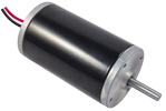
Figure 1. Vex Robotics CIM Motor
This blog will show you how this motor is modeled, mathematically, using the tools on PartQuest Explore. This allows you to design with this motor and be able to accurately predict how your system will perform, all in a virtual environment. Let's start with the end, though, by first looking at a PartQuest Explore test circuit that includes a model of a CIM motor. Then, later in this blog, I will show you how the model was developed.
Video Presentation
Watch this if you want a quick overview of this blog.
PartQuest Explore CIM Motor Test Example
The PartQuest Explore schematic in Figure 2 shows a CIM motor in a test configuration. This is a live view of the design -- you can move the probes and see different signals of interest. When you compare this with the measured data provided by Vex Robotics (see Figure 3 below), under the same test conditions, you will see that it matches quite well.
Figure 2. CIM Motor Test Circuit
Ideal voltage source vs. battery
Note that the electrical power supplied to the motor is from an ideal 12-volt DC source. This corresponds to a lab bench instrument that regulates the voltage to ensure it stays constant at the set value (12 V). Any electrical current that is necessary will be supplied to support keeping the voltage at 12 V.
This is good, for this controlled test scenario, but this is not the same thing as using a battery to power the CIM motor! The batteries that are typically used in FRC competitions are nominally 12-volt batteries, but the actual voltage across the battery terminals is a function of when the battery was last charged as well as the electrical current being drawn from the battery at any particular time. As a current load is drawn from the battery, the voltage drops. Consequently, a battery's voltage can be as high as about 12.6 volts, under no-load conditions, and can drop as low as about 6 volts under heavy load.
Mechanical load
Also notice the mechanical load configuration of this test circuit. The block with an "ω" on it is a source that will supply any torque that is necessary to keep the mechanical shaft velocity (in radians per second) of the motor to a specified value. This model is controlled by the chain of signals to the left in Figure 2, causing the shaft speed to be swept from 0 rpm up to 5,330 rpm; over time, from 0 seconds to 5,330 seconds. Thus the time axis of the plots and the rpm of the motor correspond.
View in explore.partquest.com
You can use this test circuit yourself. Just click on the "Edit in PartQuest Explore" button. This will open the design for viewing. Click on the "Copy" button to edit the design for your own use (you may need to login or create a free account). You can change the voltage or loading conditions or make any other variation of the circuit that you wish and re-simulate the circuit. Move the probes to see results.
Why Model a CIM Motor?
Motors are used to accomplish a job -- driving the wheels or tracks to make the robot move, or spinning a wheel as part of a shooter mechanism, or driving a winch to enable the robot to scale a wall. Any robot design using a motor has to answer several questions: Will the motor be able to provide the necessary force or torque for the mechanical load? How much current will the motor draw under load? Will the breaker be tripped? Will the motor burn up? What gear ratio gives us the right tradeoff of torque vs. speed?
Like all DC motors, the CIM motor provides performance that varies significantly as a function of the electrical source (voltage and current), and mechanical load (speed and torque). These are represented by the multi-dimensional graph below. The measured data in Figure 3, provided by Vex Robotics, characterizes the performance of this motor, across these variables.
Answering the above questions depends on determining where on these curves the motor is operating. But this isn't easy to do, as the operating point changes while the motor is being used, and all of the variables interact.
This remainder of this blog will show you how to encapsulate this information into a mathematical model, then use it to predict CIM motor performance under conditions that are different from the test data.
Measured Data for a CIM Motor
This graph shows the performance of a CIM motor as a function of mechanical shaft velocity in RPM. This corresponds exactly to the PartQuest Explore test circuit shown above -- with an ideal 12 volt voltage source and a swept shaft velocity load.
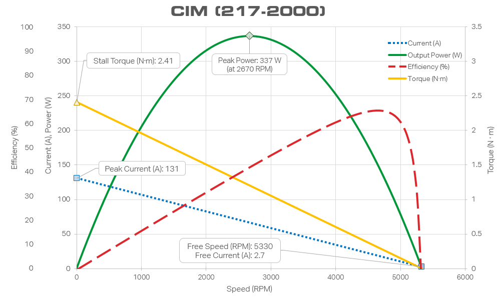
Figure 3. CIM Experimental Data
DC Motor Equations
This model uses the following simultaneous differential equations, shown below in Equation 1 and Equation 2.
(Equation 1)
(Equation 2)
Below are the sign conventions for the main variables: voltage, current, angular velocity, and torque.
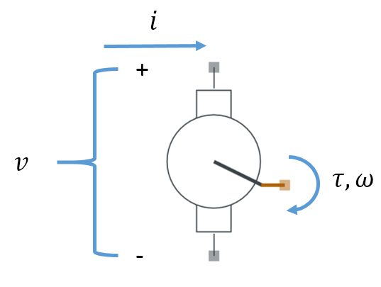
Figure 4. Motor Symbol With Sign Conventions
Note that torque () is defined as a positive value when applied to the motor, not by the motor. Consequently, from the perspective of the motor model, a positive current produces a negative torque.
The variable names are defined as:
| Symbol | Description | Units |
Type |
Typical value |
|---|---|---|---|---|
| Motor shaft torque | Dependent |
|
||
| Motor torque coefficient -- torque produced by motor current | Coefficient |
|
||
| Motor winding current | Independent | |
||
Viscous damping coefficient |
Coefficient |
|
||
| Motor shaft speed | Independent |
|
||
| Motor rotor moment-of-inertia | Coefficient |
|
||
| Motor winding voltage | Dependent |
|
||
| Motor voltage coefficient -- EMF produced by motor shaft velocity | Coefficient |
|
||
| Motor winding resistance | Coefficient |
|
||
| Motor winding inductance | Coefficient |
|
Table 1. Model Variable Names and Descriptions
The EMF (electro-motive-force) -- also known as "back EMF" -- is the voltage produced by the motor when it is operating as a generator. Spinning the shaft of a motor, by applying mechanical work, produces a corresponding voltage on the winding terminals.
There is a good discussion on the Chief Delphi forum regarding the relationship between the torque coefficient (Kt) and the voltage coefficient (Kv). Under certain modeling assumptions, these two values should be identical. The model here lumps certain losses into the Kv term, which causes the value of Kv to be larger than Kt.
This set of equations has sufficient flexibility to accurately model the CIM motor. Fitting this model to the measured data, by determining specific values for the coefficients, is the task of the next section.
Shaft Speed: RPM vs. Radians Per Second
The shaft speed, represented by in Equation 1 and Equation 2, is in units of radians per second. It is also common for shaft speed data to be represented in units of RPM (revolutions per minute). This is the case, for example, on the x-axis of Figure 3. It is useful to be able to convert between these units.
Here is an example of converting the maximum CIM motor speed, as determined from Figure 3, from 5330 [RPM] to 558.15 [radians per second]:
Determining Model Coefficients
Steady-state Coefficients
The data in Figure 3. are for steady-state operation of the motor -- each data point is obtained by running the motor at a fixed speed long enough for all transient behavior to settle out. Then all of the other variables (current, voltage, and torque) are measured and recorded. This is repeated for each motor speed in the data set. The entire original data set can be downloaded here. A spreadsheet with all of the calculations below can be found here.
Since this motor is in steady-state for each data point, the time derivatives of current and angular velocity are zero:
(Equation 3)
(Equation 4)
Therefore, Equations 1 and 2 reduce to:
(Equation 5)
(Equation 6)
Calculate 
Using the data point where (Speed RPM = 0), we see that the torque is 2.41 [N*m] and the current is 131 [A]. We can then solve Equation 5 for
Note that torque () is defined as a positive value when applied to the motor, not by the motor. The data set provided by Vex Robotics is therefore a set of negative torque values, from the perspective of the model.
Calculate 
Also using the data point where (Speed RPM = 0), we see that the voltage is 12 [V] and the current is 131 [A]. We can then solve Equation 6 for
Calculate 
Now that we have a value for , we can plug in values for torque, current, and speed, for each data point supplied, to determine D for each data point in the data set. This set of values can then be averaged to determine a good value for D.
(Equation 7)
Calculate 
Now that we have a value for , we can plug in values for voltage, current, and speed, for each data point supplied, to determine
for each data point in the data set. This set of values can then be averaged to determine a good value for
.
(Equation 8)
Rotor MOI J
The moment of inertia (MOI) of the motor's rotor (J) affects how quickly the motor can spin up or down. There is a good discussion on calculating the motor moment of inertia on the Chief Delphi forum. This analysis found the value of J to be:
Winding Inductance L
The inductance of the motor's winding (L) affects how quickly the electrical current in the winding can increase or decrease. There is a good discussion on calculating the motor winding inductance on the Chief Delphi forum. This analysis found the value of L to be:
Implementing the Model in VHDL-AMS
A model that corresponds to the equations described in this blog can be created for use with the PartQuest Explore tools. This is accomplished by using the IEEE standard 1076.1 VHDL-AMS language, which is well-supported by the PartQuest Explore simulator. The symbols in the schematic, above, each have a corresponding model associated with them. To see the source code of the model, simply click the right-mouse-button on the symbol and select "View/copy model." You will then see a view of the model text, which you can also copy, save, and edit to create a new model.
The VHDL-AMS language looks like a programming language, but it is primarily a modeling language. It allows you to express the equations of your model as a set of simultaneous, nonlinear, differential equations. You don't have to write any software to solve the equations, you only have to express the equations in a form that the simulator can interpret.
Use This Model
You can use this model to create electro-mechanical circuit diagrams of your own and predict how your system will behave, both electrically and mechanically.
Copy the design in Figure 2, as described above. Click on the motor model with your right-mouse-button and select "Add Favorite" to add this model to your list of favorite models. Then you can create a new schematic that uses this model.
Example: CIM Motor Spin-Up with Inertial Load
This example shows how this model can be used in a more realistic scenario. Here we see the CIM motor, powered by a battery, driving an inertial load through a gearbox. This is a good example of a mixed-discipline network. The black wires are electrical nodes and the brown "wires" are mechanical nodes. The PartQuest Explore simulator will solve the network of equations that these represent, ensuring conservation of energy by satisfying Kirchoff's current and voltage laws, as well as Newton's laws for sum of forces (actually torque in this example).
The inertial of the wheel corresponds to a 3.875 inch Banebot wheel. The gear ratio corresponds to a Toughbox Mini (12.75:1). The inrush current for the motor is dependent on the mechanical load. Notice the units on graphs of the brown nodes (radians per second).
Figure 5. CIM Motor Spin-Up With Intertial Load
You can copy this design and change the parameters of the load and/or gearbox to experiment with electrical loading and determine how long it will take for the wheel to spin-up to the desired speed. You can also change the motor-type parameter of the motor to choose a different FRC motor.