Sensor Modeling and Signal Conditioning Circuit Design for Mechatronic Systems

PartQuest Explore provides a great design platform for sensor signal conditioning circuits, as well as for verifying sensor systems in the context of their external applications. A key feature PartQuest Explore that makes this possible is the ability to create a “just right” model of the sensor itself. This can be a detailed physics-based model that captures both the internal behavior and the electrical interface characteristics of the sensor, to accurately represent its interaction with the signal conditioning circuit. Or it can be a “graphical model”, based on transfer functions or abstract math-blocks, to be used for performance and stability assessment of the system in which the sensor is placed. The IEEE Standard VHDL-AMS hardware description language covers the broad range of modeling capability needed to represent the sensor, the analog and digital aspects of the signal conditioning circuit, as well as the complete mechatronic system.

 

LVDT Sensor Signal Conditioning Circuit Design

An LVDT, or Linear Variable Differential Transformer, is a translational position sensing component. It is essentially a transformer with position-dependent variable coupling between its primary and two secondary windings. These are passive components, so active signal conditioning is required to use them. This includes an oscillator to drive the primary winding and a demodulator to convert the secondary output signals into a variable “DC” voltage level proportional to the mechanical displacement.

Macro Sensors™ PR-750 LVDT Series

The schematic below shows a complete LVDT sensor system. In the upper left, a force source, mass, damper and spring represent a simple dynamic mechanical load. The core of the LVDT (highlighted in light green) is attached to the connection point that represents the load position. The user can specify the LVDT windings’ electrical parameters (Rp, Lp and Rs), as well as its sensitivity and mechanical stroke length. Inside the model, these values are converted into the fundamental physical equations that define the electrical behavior of the device.

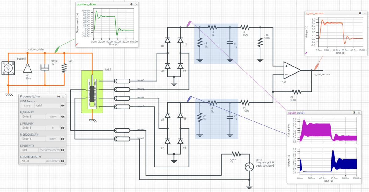
Position sensing system with LVDT and signal conditioning circuit

The design focus is on the demodulator circuit, which includes two full-wave rectifiers, two low pass RC filters (highlighted in light blue), and a differential amplifier circuit. The simulation results show the sensor’s output response (orange waveform) resulting from a 70 mm step of the underdamped mechanical load (green waveform).

The unfiltered outputs of the rectifiers (magenta and blue waveforms) clearly illustrate the variable coupling that occurs, between the constant amplitude primary input signal and the two secondary winding outputs, as the core position changes over time. The low pass filters must be designed to remove the 2.5 kHz oscillator signal, but pass all the important frequency content of the actual mechanical position, such as vibration modes that need to be sensed or the overshoot and ringing seen in this example.

You can view the “live” version of this LVDT design here. You can move waveform probes around and look at any signal in the system, or make a copy of this design and modify/add/delete components and run new simulations to see the effect of those changes. You can also view the open-source VHDL-AMS model of the LVDT, or any other component used in the design.

 

Temperature Sensor in a Thermostat Control System

An alternate method for sensor modeling in PartQuest Explore is to graphically assemble a set of transfer-function or math-block models, to represent all the behavior of the device that is relevant to the system design objective. A graphical model of a temperature sensor is shown in the schematic below, where a thermal connection point (red net) on the left can be attached to any thermal network to read its temperature. The electrical connection point (black net) on the right drives the sensor output voltage and current into any external signal path or conditioning circuit.

“Graphical Model” of a temperature sensor

All of the intermediate math-blocks operate on generic continuous quantities, and model the sensor’s fundamental static and dynamic characteristics. From left to right, this includes a low-pass filter with user specified pole frequency set to 0.1 Hz, which operates on the instantaneous value of the sensed temperature. The filter output goes to a gain stage, with gain value set to 0.01. This defines the sensor’s static sensitivity as 0.01V/degree-C. A fixed bias value of 0.1 is added with a summing block, to set the output voltage level to 0.1V at temperature 0C. The limit function keeps the output open-source voltage between 0.0V and 1.5V, and the resistor provides an effective 1.5kOhm output impedance to complete this sensor model.

PartQuest Explore provides a library of “Technology Converters”, like the temperature-to-continuous-quantity and the voltage-from-continuous-quantity converters used in the graphical temperature sensor (the left-most and right-most blocks, respectively). These converters allow our math-block models to operate on any physical nature or type of quantity, such as current, pressure, torque, magnetic flux, etc., and therefore support graphical modeling of almost any type of sensor. To learn more about using these converters, please see this blog and associated video.

The same temperature sensor is included in the thermostat controlled coffee cup heater shown in the schematic below. (Note: This schematic is "Live", you can move probes around to see other signals and click on components to see their parameter values). This closed loop system also has an analog amplifier stage, a digital thermostat with a voltage threshold or trip-point, a clock to set the sample-rate and a flip-flop to preserve the heater switch state between samples. A 12V automotive battery provides power to the heating element when the heater switch is closed. The resulting heat-flow enters a thermal network that models the thermal behavior of the coffee-cup itself. This includes conduction and radiation heat transfer to the ambient environment, as well as heat capacitance.

Automotive coffee cup heater with thermostat temperature control

The light blue waveform shows the thermostat output state that controls the heater switch, as it regulates the temperature of the coffee cup (red waveform). Inside the temperature sensor model, the effect of the low-pass filter can be seen by comparing the instantaneous temperature value (green waveform) and the filtered output value (magenta waveform). The smoothing and delay effect of this filter, which represents the internal time constant or detection speed of the sensor itself, can have a significant impact on the overall loop temperature regulation.

In the waveforms shown in the graph below, the red waveform is the coffee cup temperature as shown in the design above, with the sensor bandwidth set to 0.1 Hz, and the thermostat temperature sampling period set to 1 second. The blue waveform corresponds to the use of a faster sensor (1 Hz bandwidth) and faster temperature sampling (0.2 second period). This type of “in context” assessment of system performance can be very helpful in choosing the right sensor for a particular application.

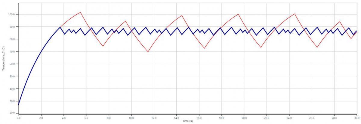
Compare temperature regulation for fast vs. slow sensor

You can view the “live” version of this Coffee Cup Heater design here. As with the LVDT example discussed previously, you can interact directly with the live design, or make a copy and modify it as desired, then run new simulations to see the results.