Managing PWM Waveforms, Part 1 - Data Reduction

This is the first part of a three-part series on special handling of PWM waveforms. The first two parts deal with the large amount of data involved. The last part deals with precise characterization in the presence of switching cycle “noise.” I am honored to post this article, which was created by one of our talented community members, a modeling and simulation expert and my friend, Norm Elias.

Large amounts of data, i.e., large numbers of time points, result from simulating milliseconds of switch-mode operation with microseconds per switching cycle. Even if all of your software applications can handle the large files, those files can be an inconvenience. Fortunately, there is an easy way to reduce the data by sampling the time points. I’ll use the series R-L-C design in Figure 1 to describe and demonstrate the data reduction procedure.

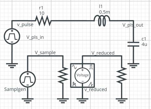
Figure 1 Introductory Example, Series Resonant Circuit

This design can be found here.

In a nutshell, I’m describing a pre-process simulate/post-process procedure. The pre-process step adds a sampling strobe to the original design. The post-processing step is a short series of Excel edits using the sawtooth strobe to sample the waveforms. In  Figure 1, the strobe is supplied by a voltage pulse source named Samplgen. You configure it to produce a sawtooth waveform as shown in Figure 2. The sawtooth generates uniformly spaced sampling times starting at t=0. Negative going pulses make it easy to locate the strobe samples.

Figure 2 Sampling Voltage

In this example, I’m simulating the R-L-C response to a 50% duty cycle pulse. When the simulation is completed, I download all waveforms of interest plus the sampling sawtooth as shown in Figure 3. To open the waveforms in Excel, I click the box that appears at the lower left of my screen and select Open as shown in Figure 3.

Figure 3 Simulate and Export Waveforms to Excel

The post-processing in Excel is a one-time event involving the full set of original time points. It’s a cookbook procedure that follows this recipe:

• Copy all waveforms into a single spreadsheet
• Optional: Reduce the header to one row
• Sort all rows by the sawtooth (viz., v_sample), largest to smallest
• Scroll down to the first row with v_sample < 0.0
• Delete all rows from there down
• Sort all rows by the time value, Smallest to Largest
• Save the result

Figure 4 compares the V_pls_out waveform before and after this post-processing step. The Excel operations reduce the table from 6,901 time points to 201--a 97% reduction.

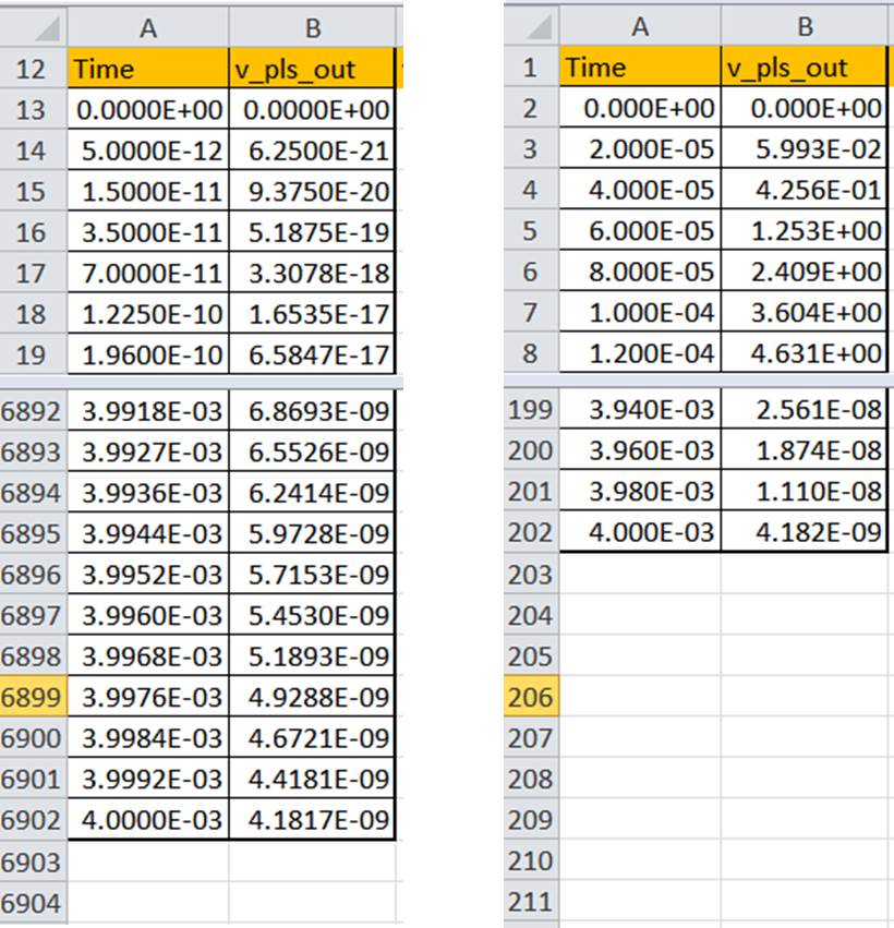
A) 6,901 Time Points                                                                                        B) 201 Samples

                                                                               Figure 4 Sample the Waveforms in Excel

The next thing I’m going to do is to put this waveform right back into the simulation so I can compare the 201 time point representation to the original 6,901 time points of V_pls_out. The same technique can be used in a development project to compare revised designs or to analyze a variety of signal processing schemes. The key ingredient is the voltage source named v_reduced in Figure 1. This is a voltage function generator, which I selected from the panel of Analog Electronics components. I’ve selected the table mode as shown in Figure 5. To place the 201 time and V_pls_out, I copy the values in Excel, open the properties menu of the function generator, select any cell after the first row, and paste the entire waveform with a single click. When I run the simulation, the function generator will output the saved V_pls_out waveform.

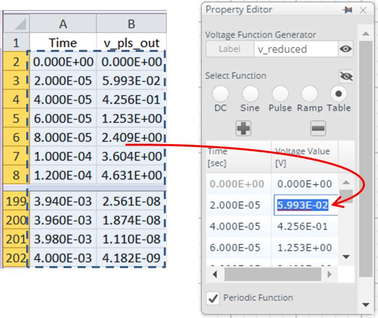
Figure 5 Copy and Paste Into a Function Generator

Figure 6 compares the 201 point waveform to the original simulation result. I’ve simulated two complete cycles of the V_pls_out pulse. With the “Periodic” box checked in the function generator menu (See Figure 5), V_reduced repeats the pulse in the second cycle. The first cycle of V_reduced appears to match the original V_pls_out waveform exactly until you zoom in and look closely. The magnified view in Figure 6 shows V_reduced as a very good piecewise linear approximation that matches exactly at the sampling points.

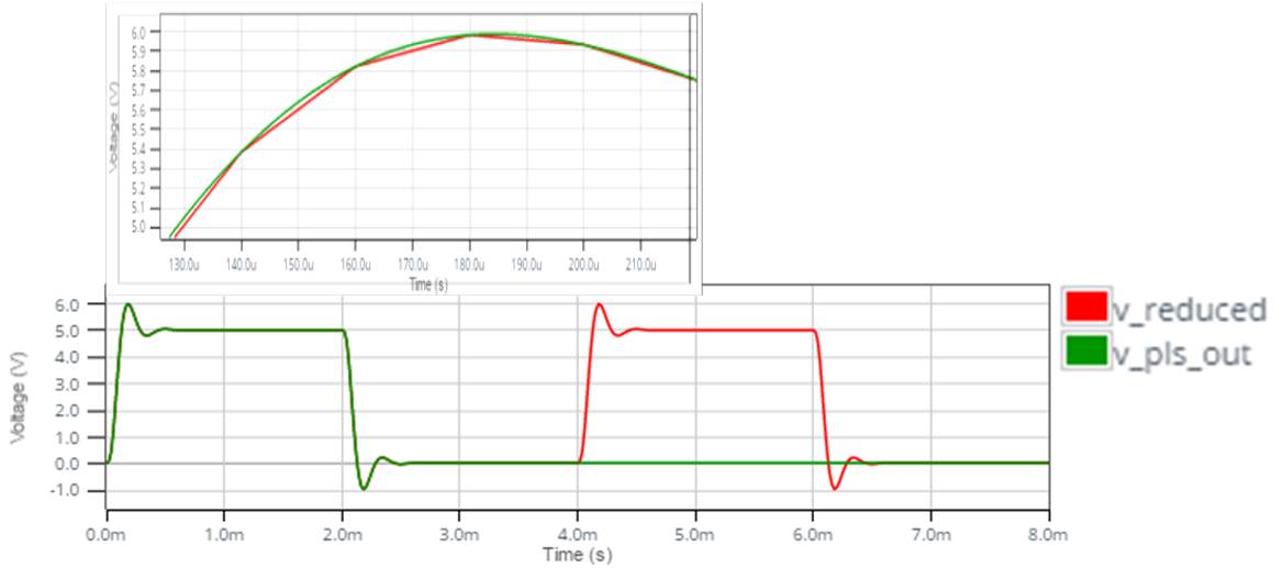
Figure 6 Compare Sampled (Reduced) and Original Waveforms

Sampling theory says that a waveform limited to a bandwidth of f ≤ f_max can be regenerated exactly at all time points if it is sampled at a uniform rate equal to or greater than twice f_max, i.e. at f_smp (= 1/T_smp) ≥ 2*f_max [C. E. Shannon, “Communication in the Presence of Noise,” Proc. I. R. E., vol. 1949]. For the R-L-C example, a frequency analysis shows that V_pls_out is 20dB down at f_max = 12 KHz. For f_smp = 2*f_max = 24 KHz, the 4ms pulse can be regenerated from as few as 24 KHz * 4ms = 96 samples.

The 201 samples used here are more than enough. However, a PWM waveform, such as that sketched in Figure 7, would require a much larger set of samples because of the switching cycles present. For a 20us switching cycle that must be resolved to 1us/sample, at least 4,000 samples would be needed to store 4ms of simulation results. A 10us switching period would require 40,000 samples. These are only a small fraction of the half-million time points typically seen in the original simulation results, but they exceed the practical limits of the function generators.

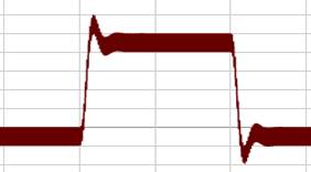
Figure 7 A Pulsewidth Modulated Waveform (mocked up by adding the sawtooth V_sample to the R-L-C output V_pls_out)

The solution to this problem is the topic of Part 2 of this series. Keep a watch for that blog.